# redpitaya-MCPHA
A Multi-Channel Pulse-Height Analyser for the [RedPitaya FPGA board](https://redpitaya.com/de/)
for physics laboratory courses
## Overview
The RedPitaya is a small, credit-card sized single board computer with a dual-core ARM Cortex-A processor
and a XILINX Zynq 7010 FPGA. The board contains two fast ADCs and two DACs with 14 bit resolution running
at a sampling frequency of 125 MHz. Extension connector provide general purpose IO pins with
slow analog inputs and outputs and support for serial bus interfaces like I²C, SPI and UART.
The system runs under Ubuntu Linux, which provides network access and supports a wide range of
applications running on the board.
Many laboratory instruments like oscilloscopes, logic analyzers, Bode plotters or a multi-channel pulse-height
analyzer can be realized on this board by simply changing the FPGA image and the Linux application.
{width=800px}
The MCPHA application for the RedPitaya by Pavel Demin provides a multi-channel pulse-height analyzer and
consists of an FPGA image and a server process running on the RedPitaya board. A client script controls
the server and pulls the data to the client computer.
### Files:
- *README.md* this documentation
- *mchpa.py* client program
- *redPoscidaq.py* a simple oscilloscope and daq client using the mcpha server
- *examples/* recorded spectra
- *examples/peakFitter.py* code to find and fit peaks in spectum data
- *read_npy.py* a simple example to read waveforms saved in *.npy* format
- *redP_mimocorb.py* runs *redPoscdaq* as a client of the buffer manager *mimoCoRB*
- *run_daq.py* script to strat the *mimoCoRB* application
- *setup.yaml* coniguration script defining the *mimoCoRB* application
- *modules/* and *config/* contain code and configuration files for the *redP_mimoCoRB* application
- *mcpha.ui* qt5 graphical user interface for *mcpha* application
- *rpControl.ui* qt5 tab for *redPosci* application
- *mcpha_daq.ui* qt5 tab for oscilloscope with daq mode
- *mcpha_gen.ui* qt5 tab for generator
- *mcpha_osc.ui* qt5 tab for oscilloscope
- *mcpha_hst.ui* qt5 tab for histogram display
- *mcpha_log.ui* qt5 tab for message display
- RP-image directory with all files necessary to boot a RedPitaya and start the server
application based on the "small, simple and secure" linux distribution
[alpine-3.18-armv7-20240204](https://github.com/pavel-demin/red-pitaya-notes/releases/tag/20240204)
- utility scripts in the sub-directory *helpers/*
## Credit:
*mcpha.py* is a fork of the sub-directory *projects/mcpha* in a project by
Pavel Demin, [red-pitaya-notes](https://pavel-demin.github.io/red-pitaya-notes), *redPoscdaq.py* represents an
extension of the oscilloscope class enabling fast restart and data export.
## Multi-Channel Pulse-Height Analyzer for the RedPitaya FPGA board
A multi-channel pulse-height analyzer produces a histogram of the heights of pulses present in a signal supplied to the input. The MCPHA project uses the FPGA on the RedPitaya board to process the digitized input signal at very high rates. A server process on the ARM processor of the RedPitaya communicates with a client process via network. The client communicates with the server, starts and stops data recording and receives and displays the data. The client is also responsible for saving data to files.
The original version by Pavel Demin has been modified to better meet the usual standards for graphics
displays in physics. A command line interface has also been added to allow easy control of important
parameters at program start.
A special version of the original oscilloscope display, *redPosci.py*, with fast transfer of data to the client for data acquisition applications is also contained in this extended package.
### Basic functionality
The *mcpha* application uses a rather simple, but straight-forward algorithm to determine the
height of pulses. When the signal voltage of a supplied input signal starts rising, the corresponding
ADC count is stored. A second ADC value is stored when the signal level starts falling again, and the difference of these two ADC values is histogrammed. The histogram is transferred to the client upon request.
The *mcpha* application also contains a signal generator that runs independently and parallel to the
pulse-height analyzer. It provides configurable signal shapes and signal rates at the *out1* connector
of the RedPitaya board. Connecting *out1* with a (short) cable to one of the inputs *in1* or *in2*
provides input signals that can be be used to familiarize with the functionality and to benchmark
the performance.
An oscilloscope with very basic functionality to set the trigger level and direction is also provided.
The timing is controlled by the so-called decimation factor that can be adjusted using the control
in the upper right corner of the graphical window. The RedPitaya samples data at a constant rate
of 125 MHz, and the decimation factor determines how many samples are averaged over and stored
in the internal ring buffer. This reduces the effective sampling rate accordingly. Only decimation
factors corresponding to powers of two are allowed. An example of randomly occurring exponential
signal pulses at an average rate of 10 kHz with a fall time of 10 µs is shown below; there is significant
signal overlap in this case, making pulse-height detection more complex.
{width=800px}
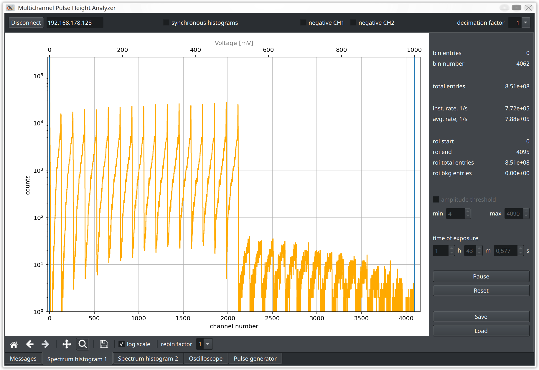
A spectrum of such pulses is shown below for input pulses at multiples of 62.5 mV between 62.5 mV
and 500 mV. The overlap of signal pulses leads to wrong pulse-height assignments below the actual
voltage and to entries above 500 mV when pulses become indistinguishable and therefore add up
to a single detected pulse.
{width=800px}
Note that spectra and waveforms are plotted with a very large number of channels, well exceeding
the resolution of a computer display. It is therefore possible to use the looking-glass button
of the *matplotlib*window to mark regions to zoom in for a detailed inspection of the data.
## Oscilloscope and data recorder
The script *redPosci.py* relies on the same server and FPGA image as the pulse-height analyzer.
The *oscilloscope* and *generator* tabs provide the same functionality as in *mcpha.py*.
In addition, however, there is a button "*Start DAQ*" to run the oscilloscope in data acquisition
mode, i.e. continuously. A subset of the data is shown in the oscilloscope display, together with
information on the trigger rate and the transferred data volume. A configurable user-defined function
may also be called to analyse and store the recorded waveforms.
It is possible to transfer data over a one-Gbit network from the RedPitaya with a rate of 50 MB/s
or about 500 waveforms/s.
Two examples of call-back functions callable by redPoscdaq are provided with the package
- redP_consumer()
calculates and displays statistics on trigger rate and data volume
- redP_mimocorb()
provides an interface to the buffer manager *mimiCoRB* for more advanced data analysis tasks
requiring multiple processes running in parallel. A simple *mimoCoRB* setup is also provided
and can be started by *./run_daq setup.yaml*; modules and configuration files for a pulse-height
analysis of signals are contained in the subdirectories *modules/* and *config/*, respectively.
## Installation
The sub-directory *RP-image* contains files to be transferred to a SD card for the RedPitaya board.
Proceed as follows:
- copy the contents of the directory *RP-image* to an empty SD card formatted as VFAT32.
- connect the RedPitaya to the network via the LAN port
- insert the SD card in the RedPitaya and connect the power.
The RepPitaya directly starts the *mcpha* server application, requests an IP address via DHCP
and waits for the client program to connect via network.
On the client computer, download the client software:
- clone the *mcpha* repository via `git clone https://gitlab.kit.edu/guenter.quast/redpitaya-mcpha`
- change directory to the installation directory and start the graphical interface of the client
software via `python3 mcpha.py` on the command line.
The application program *mcpha.py* takes care of initializing the processes on the RedPitaya board
through the server process, initiates data transfers from the RedPitaya board to
the client computer and provides several tabs to visualize data, generate test data and
to store the acquired spectra.
### Network connection to the RedPitaya Board
Connecting to the RedPitaya with a LAN cable is the recommended way of access. The RedPitaya
requests an ip-address via the dhcp protocol and becomes accessible under the name *rp-xxxxxx*,
where *xxxxxx* are the last six characters of the ethernet MAC address.
If a usb-to-ethernet adapter is used and a dhcp server on the client computer is enabled for the
interface, a one-to-one connection of the RedPitaya to a host computer can easily be established;
use the name *rp-xxxxxx.local* in this case. How to set up a *dhcp* server for a usb-to-ethernet
adapter depends on the operating system used on the client; please check the relevant
documentation for your system.
## Usage
First, boot the RedPitaya with the proper SD card inserted. This starts the FPGA code
and the server process on the RedPitaya board.
Then, on the client side:
- start the client program via `python3 mcpha.py`
- in the graphical interface, enter the network address of the RedPitaya in the
field next to the orange button and click *connect*;
watch out for connection errors in the *Messages* tab!
The message "*IO started*" is displayed if everything is ok, and the address turns green.
- click the *oscilloscope* tab, check the trigger level and then start the oscilloscope
to see whether signals are arriving at one or both of the RedPitaya inputs.
Adjust the *decimation factor* in the top-right corner of the main display to ensure
that the sampling rate is high enough for about 50 samples over the pulse duration.
- if no signal source is available, you may click the *generator* tab, set the desired
signal parameters and start the generator; connect *out1* of the RedPitaya to the
input *in1* with a (short) cable and then check for the presence of signals in
the *oscilloscpe* tab.
- now click the tab *spectrum histogram 1*; adjust the amplitude threshold and time
of exposure, then click the *Start* button and watch the spectrum building up.
- when finished, use the *Save* button to save the spectrum to a file with a
meaningful name.
## Helper scripts
The directory *helpers/* contains helper scripts to read and visualize data from
files written by *mcpha.py*, for both spectrum histograms and exported waveforms.
Note that presently mcpha.py exports data in human-readable format using
*numpy.savetxt()*.
> *generate_spectrum_input.py* is a script to to generate input spectra for the signal
generator of mcpha.py The convention is to use 4096 channels for a range from 0 to 500 mV.
Pulse heights are drawn randomly from this spectrum, and pulses are formed according to the
frequency and the rise and fall times specified in the graphical interface. The signals are
available at the *out1* connector of the RedPitaya board.
>
> Pulses can be generated at a fixed frequency, or with random timing corresponding to a
Poisson process with a mean pulse rate given by the chosen frequency. The latter option is
useful to study "pile-up" effects from overlapping pulses.
> *read_hst.py* illustrates how to read and plot spectrum data exported by mcpha.py.
> *read_osc.py* demonstrates how to read and plot waveform data exported from the
oscilloscope tab of mcpha.py.
## Examples
The directory *examples/* contains some spectra recorded with *mchph.py* and the Python
program *peakFitter.py* to find and precisely fit peaks in recorded spectra. An example is
shown here:
{width=800px}
## License
Like the original code by Pavel Demin, this open-source code is provided under the MIT License.
## Project status
This project has been developed for experiments in the physics lab courses at the Faculty of Physics
at Karlsruhe Institute of Technology. The code is already public, but presently still under test.